
INTRODUCTION TO FASTAI
What Is FastAI?
It is a research lab started by two people: a former Kaggle President and the other a well-known AI expert. Its mission is to make AI accessible to everyone. Fast.ai can be described as a course-bundled research lab, an easy-to-use Python library with a vast community. Their library wraps popular libraries for common workflows of deep learning and machine learning and provides a user-friendly interface.
More importantly, the “top-down” approach follows.
“Top-down” is exactly like the way a sport is learned. We start by trying to play it without having to worry about rules. Once we are confident, we learn one by one of the rules and the tricks.
Similarly, fast.ai lets us create a model using just a few lines of code. After that, we can further improve it.
FastAI is designed to simplify neural network training. It is based on research into the best practices in deep learning. Has support outside the box for:
- Vision
- Text
- Tabular data
- Collaborative filtering
FastAI is created on top of Pytorch and hence includes some pre-trained models such as resent18, resnet34, resnet50, resnet101, resnet152 (each with different layers) as densenet121, densenet169. It is complementary to Pytorch, a Python-based deep-learning library used in computer vision and neural network models.
Controlling Resources
You would need to use an Nvidia GPU. Unless you own a gaming PC, you’re unlikely to have an Nvidia GPU. Even if you’ve got an Nvidia GPU, you may need to download any data to train models from the internet. The best option is to use a GPU in the Cloud.
Here are a few options:
CRESTLE
Crestle is the easiest starter option. It costs about 0.60 USD an hour. You don’t have to set up anything, only start learning.
PAPER SPACE
Paperspace has an array of GPU options to choose from. The starting option is cheaper and more reliable than Crestle. The downside is you’d have to spend around an hour doing the initial setup. If you don’t have some Linux experience, it could be not easy.
AWS AND GCE
Both of these cloud providers have a wide range of GPU options, and in the long run, they might be more cost-effective than Paperspace. You could also use free credits to sign up—Google for “FastAI AWS” or “FastAI GCE.”
GOOGLE COLAB
You can get a GPU for free using Google CoLab. Running fast.ai on CoLab is challenging, as it is mainly built for Tensorflow (Google’s deep learning toolkit). If you have time to experiment with that, you might try to make it work for fast.ai.
What Speeds Up FastAI Training?
It includes an OO class, encapsulated preprocessing, augmentation, test, training, and validation sets, multi-class versus single classification versus regression, as mentioned in the documentation in FastAI. Along with architecture model choice. Thus FastAI can determine the best architecture, preprocessing, and training parameters for that model, for that data, mostly automatically. And finally, it became more productive and made far fewer mistakes because it automated everything that could be automated. For example, it tends to customize models more difficult for Keras, especially during training. More importantly, the static computing graph on the back-end, together with Keras’ need for an extra compile() phase, means it’s hard to customize a model’s behavior once it’s built and FastAI is much quicker in this case.
What Benefits Does the FastAI Library Have Over Other Libraries?
Because of fewer codes written by AI developers, everything is much more comfortable with FastAI. As the documentation says, at the same time, FastAI delivers flexibility, speed, and ease of use. It offers many features and functionality, which makes developers customize the high-level API without engaging in low-level API parts. One example of this customization is DataBlock, which allows you to load the data in detail. As FastAI explains, DataLoader class loads both the training and the validation data classes. Besides, the process of using validation data sets while training the data would make the job easier. Beginners working with this library, therefore, use available functions and start customizing models. The figure shows four fields of applications, including vision, text, tabular, and collaborative filtering, each of which is used for different purposes.
Step 1: Install fastai in the Python service
The first step in the tutorial is to install the fastai library. To get started, navigate to the Python service to install the fastai library from PyPi as shown in the example below. There are many different approaches to installing the library but in this instance we install the latest version of the fastai and nbdev package from PyPi, required to run the first notebook in the fastai course.
Step 2: Configuring and starting Jupyter
In the Jupyter service page there are three different modes that can be configured.
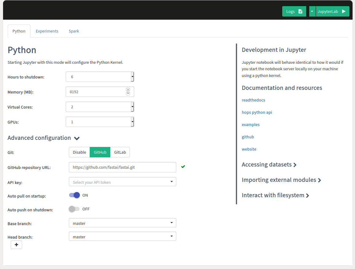
Firstly, there is a Python tab, in which configuration for the Python kernel, such as Memory/Cores/GPUs is set and optionally a git repository can also be configured that should be cloned when Jupyter starts up. This is the kernel that we are going to use in this tutorial.
Secondly, in the Experiments tab the PySpark kernel is configured. If you want to enable all the features in the plattform regarding, experiment tracking, hyperparameter optimization, distributed training. See HopsML for more information on the Machine Learning pipeline.
Thirdly, for general purpose notebooks, select the Spark tab and run with Static or Dynamic Spark Executors on Spark or PySpark.
The image below shows the configuration options set for the Python kernel. As working with larger ML models can be memory intensive make sure you are configuring the Memory for the kernel to be at least 8GB, then set GPUs to 1 to allocate a GPU that should be accessible for the kernel and set the git configuration to clone the fastai git repository https://github.com/fastai/fastai.git to get access to the notebooks.
Step 3: Start the Notebook Server
Once the configuration has been entered for the Python kernel, press the button on the top that says JupyterLab to start the Notebook Server. Keep in mind that it may take some time as resources need to be allocated for the Notebook Server and to clone the git repository. The image below demonstrates the process of starting Jupyter.
Step 4: Inspecting the GPU
The Jupyter Notebook Server will now have been allocated a GPU which you can use in the Python kernel. To check the type and specifications of the GPU, open a new terminal inside Jupyter and run nvidia-smi. We can see that in this instance we have access to a P100 NVIDIA GPU.
Step 5: Start using fastai by following the course material
Now you’re all set to start following the course material that fastai provides. To make sure the GPU is being utilized you can leave a terminal window open and run nvidia-smi -l 1, which will print out the GPU utilization every second while you are running the training in the notebook.
In the example below, the first notebook lesson1-pets.ipynb in the fastai course is executed.
There are many articles on fastai v1. But since the developers have created v2 from ground up, there are very little information on the same, except for the official documentation, which, in my personal experience, is not very much detailed.
Anyways, you can go to their official documentation
They have divided the framework into 3 sections: tabular, vision and text. Tabular ML covers the machine learning problems where we have a list of features for each user or device or as we call them technically, samples. Vision covers the problems which have images as the dataset and we might have to do classification, or semantic segmentation or object detection. Text covers the sections where we want to do natural language processing.
In this article, I am going to explain only one component, vision.
Vision: A general pipeline
- Import Library
import torch
import fastai
import numpy as np
import matplotlib.pyplot as plt
from pathlib import Path
from PIL import Image
from tqdm import tqdmfrom fastai.vision.all import *
from fastai.vision.augment import *
device = torch.device("cuda:0" if torch.cuda.is_available() else "cpu")
device
This will import all the necessary libraries.
2. Create dataset generator
We can load our dataset in many ways. I will be using dataframe for creadting dataloader.
csv_path = '../input/hackerearth-holiday-season/dataset/train.csv'
train_path = '../input/hackerearth-holiday-season/dataset/train'
test_path = '../input/hackerearth-holiday-season/dataset/test'df = pd.read_csv(csv_path)
df

We will be modifying our Image column so that it becomes a direct path to image location. For that we will use function pandas.DataFrame.apply() which is very useful to modify the contents of a Data frame.
df['Image'] = df['Image'].apply(lambda x: os.path.join(train_path, x))
df
Now we have our Image column exactly how we want. Great!
For plotting the histogram for class distribution, pandas already gives us a nice command to plot it right away!
df['Class'].value_counts().plot.bar()
Now, we would like to finally create our dataloader. For that, fastai provides the class ImageDataLoaders which has an internal function from_df()
img_size = 128
augmentations = [
        Rotate(10, p=0.4, mode='bilinear'),
        Brightness(max_lighting=0.3,p=0.5),
        Contrast(max_lighting=0.4, p=0.5),
        RandomErasing(p=0.3, sl=0.0, sh=0.2, min_aspect=0.3, max_count=1),
        Flip(p=0.5),
        Zoom(max_zoom=1,p=0.5),
        RandomResizedCrop(img_size)
    ]dls = ImageDataLoaders.from_df(df=df,
                               path='.',
                               valid_pct = 0.2,
                               bs = 32,
                               device=device,
                               num_workers=0,
                               batch_tfms=augmentations,
                               item_tfms=Resize(img_size))
dls.show_batch()
fastai v2 allows multiple ways to create a data loaders apart from from_df. We can use ImageDataLoaders.from_folderwhich assumes two sub-directories in directory (mentioned in path parameter), train/ and valid/ by default.
ImageDataLoaders.from_folder(path, train='train', valid='valid', valid_pct=None, seed=None, vocab=None, item_tfms=None, batch_tfms=None, bs=64, val_bs=None, shuffle_train=True, device=None)There is another way: ImageDataLoaders.from_name_re which is useful if we have labels in image names itself. For example img_001_cat.jpg and img_742_dog.jpg .
ImageDataLoaders.from_name_re(path, fnames, pat, bs=64, val_bs=None, shuffle_train=True, device=None)There are many other modular ways to create dataloader. You can check that out in more detail, here.
So here we have some new terms. For adding augmentations to our dataset, we will create a list of augmentations such as Rotate, RandomErasing, RandomResizedCrop, Flip etc. They are pretty straightforward and quite literal to understand how each of them work.
For creating dls, we mention the target dataframe, that is, df. valid_pct denotes the percentage split for validation set, on which error rate and loss will be calculated for backward propagation.
Parameter path denotes the directory relative to which image paths are mentioned in dataframe. Since I have appended path in df column, we will simply put ‘.’ in path.
There are batch_tfms and item_tfms. item_tfms denotes the augmentation that is required for all images in training and valid set. batch_tfms denotes the augmentations that should be applied to batch on which we are training our model. That means batch_tfms is only for training data and item_tfms is for all images. (Thus we don’t need to add Resize() in augmentations defined above)
My understanding for writing these two separate augmentations:
item_tfms happens first, followed by batch_tfms. This enables most of the calculations for the transform to happen on the GPU, thus saving time.
The first step (item_tfms) resizes all images to same size (happens on CPU) and then batch_tfms happens on GPU. If there were only one transformation, we would have to apply them on CPU, which is slower.

3. Learner
learn = cnn_learner(dls,
                    resnet34,
                    metrics=[accuracy,error_rate])
learn.lr_find()
cnn_learner will return a model specified (resnet34 in this case). Metrics will be used to print the relevant information after each epoch. accuracy metric will show loss after each epoch. error_rate will show, well error rate, pretty self explanatory.

lr_find is a very good way for choosing an appropriate learning rate. Thumb of rule would be choose the lr=min_lr/10 where min_lr is the learning rate at which loss was minimum. This is because choosing min_lr might result in a slightly large lr which might diverge your loss after some epochs. For example, in this plot, I’d choose learning rate at 1e-2.
Now we fit the model using command:
learn.fit_one_cycle(epochs, lr, wd)fastai v2 has another function called learn.fit() which has the same parameters but it will fit with a fixed learning rate mentioned by the user. learn.fit_one_cycle() will use a cyclic lr type of scheduler with maximum learning rate as lr mentioned by the user. wd denotes the amount of weight decay. fastai encourages wd=1e-2. This is a classic method to reduce overfitting by introducing regularization. With vanilla SGD the weights will be corrected as:
w = w - lr * w.grad - lr * wd * wYou can also unfreeze the model by:
learn.unfreeze() # Set requires_grad=True for all layerswhich means that the parameters of the base model are now also trainable. Developers should be careful because after unfreezing the model, one should use very low learning rate. Unfreezing the model is only for fine tuning the model.
One can also set different learning rates to different parts of model after unfreezing.
learn.unfreeze()# deepest layers will have lr=1e-5, middle layers will have lr=1e-4 and layers at the beginning will have lr=5e-4
learning_rate = [1e-5, 1e-4, 5e-4]learn.fit(learning_rate, epochs=3)
4. Plots
After training we can see some useful plots.
4.a For plotting loss curve of train and validation, write learn.recorder.plot_loss()

PS: learn.recorder.plot_metrics() was used in fastai v1 but is depreciated now.
4.b Plot confusion matrix
interp = ClassificationInterpretation.from_learner(learn)losses,idxs = interp.top_losses()interp.plot_confusion_matrix(figsize=(7, 7), dpi=100)

4.c Top loss images
interp.plot_top_losses(4, figsize=(10,11))
This command shows the images that had the highest loss in training. This is pretty useful for debugging purposes.